A visual explanation of flow matching
1D denoising: a path, its prediction, and a cloud.
Demo by Donghoon Ahn
Click or drag in the plot. The red image is a prediction; the green image is where the flow ends.
Analytic 1D flow · images ordered by pixel-based t-SNE · photo averages use the scalar posterior.
Current input · xₜ
From the same initial noise to the selected final image.
Prediction · \hat{x}_1
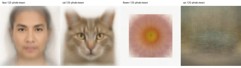
The average of all 500 photographs.
Images being averaged →
The red image is the weighted average of the photos in the cloud.
About this demo
The flow is an analytic 1D Gaussian mixture. The photos are linked to its scalar values, and the image prediction averages them using its posterior weights. These are not posteriors computed from noisy RGB pixels.
x_t=t x_1+(1-t)\epsilon,\qquad v^*(x_t,t)=\mathbb E[x_1-\epsilon\mid x_t,t]
The red arrow keeps the current velocity fixed. The teal path updates the velocity as it goes.
\hat{x}_1=x_t+(1-t)v^*(x_t,t)=\mathbb E[x_1\mid x_t,t]
The 500 photos were generated with SDXL-Turbo. Source code.